“The scientist does not study nature because it is useful; he studies it because he delights in it, and he delights in it because it is beautiful.”
Henri Poincaré
Table of Contents
- Table of Contents
- 1. Introduction
- 2. Sympy for Error Propagation
- 3. Error Propagation for Scalar Functions
- 4. Error Propagation in More Complex Functions
- 5. Error Propagation with Matrices
- 6. Frequently Asked Questions
- 7. Conclusion
- 8. External Resources for Further Learning
1. Introduction
Mastering error propagation is essential when working with experimental data, especially in fields such as physics, engineering, and other experimental sciences. In this comprehensive guide, we will explore how to perform error propagation using the Sympy library. We assume you are already familiar with Sympy basics; if not, please refer to our previous post on Sympy, How to Master Sympy.
Error propagation is the process of determining the uncertainty in a derived quantity based on the uncertainties in the input quantities. Uncertainties can arise from various sources, such as measurement errors, rounding errors, or systematic biases. By propagating uncertainties through a calculation, we can estimate the overall uncertainty in the final result, providing a more accurate and reliable understanding of our data.
2. Sympy for Error Propagation
Sympy is a Python library for symbolic mathematics. It provides tools to perform algebraic manipulations, calculus, and equation solving symbolically, making it an excellent choice for error propagation. By representing variables and their uncertainties as symbolic expressions, we can use Sympy to apply the rules of calculus and simplify expressions, ultimately determining the uncertainty in our final result.
3. Error Propagation for Scalar Functions
Let’s start with a simple example of error propagation for scalar functions.
Example 1: Addition
Suppose we have two measured values, x and y, with uncertainties dx and dy. We want to find the value and uncertainty of their sum, z = x + y.
import sympy as sp

x, dx = sp.symbols('x dx')
y, dy = sp.symbols('y dy')

z = x + y
dz = sp.sqrt(dx**2 + dy**2)
Now, let’s evaluate the expression for a specific example: x = 5 ± 0.1 and y = 10 ± 0.2.
z_value = z.subs({x: 5, y: 10})
dz_value = dz.subs({dx: 0.1, dy: 0.2})

print("Sum (z):", z_value)
print("Uncertainty in sum (dz):", dz_value)
4. Error Propagation in More Complex Functions
Example 2: Lens Maker’s Equation
Consider the lens maker’s equation for a thin lens:
f_inv = (n - 1) * (1/R1 - 1/R2)
where f_inv is the inverse of the focal length, n is the index of refraction, and R1 and R2 are the radii of curvature of the lens surfaces. We want to determine the uncertainty in the focal length (f) given uncertainties in n, R1, and R2.
First, let’s define our symbols and the lens maker’s equation:
n, dn = sp.symbols('n dn')
R1, dR1 = sp.symbols('R1 dR1')
R2, dR2 = sp.symbols('R2 dR2')

f_inv = (n - 1) * (1/R1 - 1/R2)
Now, let’s propagate the uncertainties in the input variables:
df_inv = sp.sqrt((sp.diff(f_inv, n) * dn)**2 + (sp.diff(f_inv, R1) * dR1)**2 + (sp.diff(f_inv, R2) * dR2)**2)
f = 1 / f_inv
df = abs(df_inv * f**2)
We now have expressions for the focal length and its uncertainty. Let’s calculate the focal length and its uncertainty for a specific example: n = 1.5 ± 0.001, R1 = 100 mm ± 1 mm, and R2 = -100 mm ± 1 mm.
f_value = f.subs({n: 1.5, R1: 100, R2: -100})
df_value = df.subs({n: 1.5, dn: 0.001, R1: 100, dR1: 1, R2: -100, dR2: 1})

print("Focal length (f):", f_value)
print("Uncertainty in focal length (df):", df_value)
5. Error Propagation with Matrices
In this section, we will demonstrate how to propagate uncertainties through matrix operations. We will use an example from optics.
Example 3: ABCD Matrix for a Thin Lens
Consider the ABCD matrix for a thin lens:
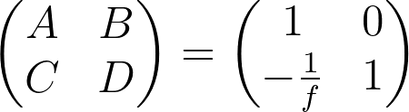
where f is the focal length of the lens. We have an input ray given by a column vector [h_in, θ_in] and want to find the output ray [h_out, θ_out] and its uncertainty.
First, let’s define our symbols and the ABCD matrix:
h_in, dh_in = sp.symbols('h_in dh_in')
θ_in, dθ_in = sp.symbols('θ_in dθ_in')

A = 1
B = 0
C = -1/f
D = 1

M = sp.Matrix([[A, B], [C, D]])
input_ray = sp.Matrix([h_in, θ_in])
Now, we calculate the output ray and its uncertainty using the matrix multiplication:
output_ray = M * input_ray
dh_out = sp.sqrt((sp.diff(output_ray[0], h_in) * dh_in)**2 + (sp.diff(output_ray[0], θ_in) * dθ_in)**2)
dθ_out = sp.sqrt((sp.diff(output_ray[1], h_in) * dh_in)**2 + (sp.diff(output_ray[1], θ_in) * dθ_in)**2)
Finally, let’s calculate the output ray and its uncertainties for a specific example. Assume h_in = 1 mm, dh_in = 0.01 mm, θ_in = 0.01 rad, dθ_in = 0.0001 rad, f = 50 mm, and df = 0.5 mm:
output_ray_result = output_ray.subs({h_in: 1, θ_in: 0.01, n: 1.5, R1: 100, R2: -100})
dh_out_result = dh_out.subs({dh_in: 0.01})
dθ_out_result = dθ_out.subs({dh_in: 0.01, dθ_in: 0.0001, n: 1.5, R1: 100, R2: -100})

print("Output ray:", output_ray_result)
print("Uncertainty in h_out:", dh_out_result)
print("Uncertainty in θ_out:", dθ_out_result)
6. Frequently Asked Questions
Q: How does Sympy compare to other libraries for error propagation?
A: Sympy is well-suited for error propagation due to its symbolic computation capabilities. It allows you to manipulate variables and expressions directly, making it easier to apply calculus rules and simplify expressions. Other libraries, such as NumPy and SciPy, are more focused on numerical computations, which can be limiting when dealing with error propagation.
Q: Can I use Sympy for error propagation in other disciplines, such as biology or finance?
A: Absolutely! Sympy’s error propagation capabilities can be applied to any field that requires the propagation of uncertainties through mathematical expressions, including biology, finance, and many others.
Q: How can I handle correlations between variables when using Sympy for error propagation?
A: In this guide, we assumed that variables are uncorrelated. However, if variables are correlated, you can include the covariance terms in the uncertainty calculations. Sympy can handle such cases, but you’ll need to adjust the expressions accordingly to account for the correlations.
7. Conclusion
In this comprehensive guide, we have explored error propagation using Sympy for scalar functions, more complex functions such as the lens maker’s equation, and matrix operations in optics. By understanding and applying error propagation with Sympy, Python users can ensure accurate and reliable results in their analyses, especially in fields like physics, engineering, and experimental sciences.
We encourage you to continue exploring Sympy’s capabilities and applying these techniques to other scenarios and calculations, further enhancing your skills and understanding of error propagation.
8. External Resources for Further Learning
-
Sympy Official Documentation: The official documentation for Sympy provides extensive information on the library’s features, functions, and usage examples. It’s an excellent resource for deepening your understanding of Sympy and its applications in various domains, including error propagation.
-
Python for Science Handbook: This comprehensive handbook by Jake VanderPlas covers various Python libraries used in scientific computing, including NumPy, SciPy, and Matplotlib. While it doesn’t focus specifically on Sympy, it provides valuable context for using Python in scientific applications, which can complement your understanding of error propagation.
-
Introduction to Error Analysis: This classic book by John R. Taylor provides a thorough introduction to error analysis and its applications in the experimental sciences. It covers the fundamentals of uncertainty, error propagation, and statistical analysis of data. Although it doesn’t focus on Sympy, the concepts presented in the book can be applied using the library.
-
Physics Forums: Physics Forums is an online community for discussing various topics in physics, including error propagation. You can find many discussions and examples related to error propagation and its applications in different fields, as well as ask questions and seek guidance from experienced users.